
Tags
Tutorial Level
![]()
EGFR Rare Mutation Detection
The major advantages of digital PCR are its precision, sensitivity, and accuracy.
Indeed, digital PCR will enable you to detect and quantify rare mutations, even when present in very low amounts: less than 1% or even 0.1% of the wild-type (WT) sequence. Thus, for the detection and quantification of rare events, such as point mutations or single nucleotide polymorphism (SNP), digital PCR is the right tool for you!
In this tutorial, we will help you to prepare and analyze a rare mutation detection experiment from A to Z.
We choose here to focus on the detection of mutations occurring on the epithelial growth factor receptor (EGFR) gene. In patients with advanced EGFR-mutant non-small cell lung cancer (NSCLC), the presence of the mutation EGFR T790M renders the standard treatment, based on first and second-generation tyrosine kinase inhibitors (TKIs), ineffective. The EGFR T790M mutation is rarely detected during the initial tumor characterization and will, most often, become detectable over the course of treatment with TKI. Thus, early detection of the appearance of this mutation is of clinical importance in directing the patient to a more effective treatment.
1. How should I design an assay to detect a rare mutation?
First of all, note that the rules for designing probes and primers are the same in qPCR and digital PCR.
The option we have chosen here is to use two different hydrolysis probes (TaqMan®), with only one set of primers. These primers will amplify the region of interest. Then one probe, labeled with a specific fluorophore (represented as a solid blue circle in figure 1), will target the wild-type, and the other one, labeled with another specific fluorophore (represented as a solid green circle in figure 1), will target the mutant allele. Before ordering your probes, please check that the fluorophores you want to use are compatible with your digital PCR system in terms of excitation and emission spectra.
Finally, according to the principles of the hydrolysis probes, you will observe the generation of a fluorescent signal when the target sequence (mutant or wild-type) is present.
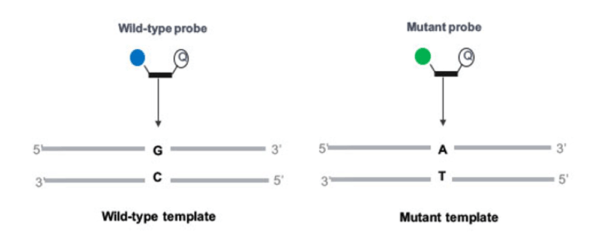
Figure 1. PCR assay using two fluorescent probes specific for the wild-type and the mutant allele respectively
2. What do I need to perform a rare mutation detection experiment?
In addition to all the tools you would require for a standard PCR experiment (microfuge tubes, vortex, microcentrifuge, pipettes, and tips, etc.), for a digital PCR experiment you will need :
- A digital PCR system and its dedicated consumables
- A PCR mastermix (please check instrument manufacturer’s recommendations) containing all the essential components to perform an experiment, including:
- A DNA polymerase
- dNTPs (desoxyribonucleotides)
- reaction buffer
- MgCl2
- and nuclease-free water
- A reference dye if necessary (please check instrument manufacturer’s recommendations)
Then you will need for this specific experiment:
- 1 primer set to amplify the EGFR T790 locus
- 1 FAM-labeled hydrolysis probe to detect EGFR WT sequence
- 1 Cy3-labeled hydrolysis probe to detect EGFR T790M mutation
- WT DNA
- DNA bearing the EGFR T790M sequence
The primer and probe sequences we used for this assay can be found in [Madic, J., Zocevic, A., Senlis, V., Fradet, E., Andre, B., Muller, S., Dangla, R., Droniou, M.E. Three-color crystal digital PCR. Biomol Detect Quantif. 2016 Nov 3;10:34-46. eCollection 2016 Dec.]
Digital PCR Principle
Since the invention of PCR by Kary Mullis in 1983, it has been a real revolution in molecular biology. A decade later, real-time PCR also termed quantitative PCR, offered the possibility of monitoring the PCR process. Until now, real-time PCR is considered as the “gold standard” for gene detection and quantification. But real-time PCR has its drawbacks such as the need for an external reference for quantification and a lack of sensitivity at low concentrations.
To further assess these drawbacks, Digital PCR was developed. The aim was to enhance the sensitivity of real-time PCR, especially in cases where detecting point mutations of low abundance in a background of wild-type DNA is required.
This technology is based on PCR amplification of DNA templates that have been randomly isolated into individual reactions. Each reaction contains zero, one or more molecules.
PCR amplification is then conducted using fluorescence dyes or probes, similar to real-time PCR.
The number of positive and negative reactions is counted by assessing the fluorescence intensity of each reaction at the end of the PCR reaction. For each reaction, a binary result is obtained explaining the term “digital”.
Finally, the proportion of positive and negative reactions is fitted into a Poisson distribution in order to obtain the absolute concentration of target molecules, eliminating the need for external references. Learn more about Poisson Distribution in Digital PCR in this detailed item: Poisson Law Computation.
A free calculator that automatically estimates target gene concentrations is also available here: Poisson Law: going further
The key feature of digital PCR is the compartmentalization of the sample. This isolates the DNA fragments from each other and then creates an artificial enrichment of low abundance sequences, leading to a higher detection level.
Finally, the dynamic range of the method is dependent on the total number of compartments generated.
Technologies to achieve a digital PCR
Until recently, digital PCR was performed using PCR plates. This process was labor-intensive and reagent consuming- limiting its use for routine analysis.
The latest advances in microfluidics enable massive automated partitioning of DNA sample in hundreds to millions of nano- or pico-liter scale compartments. Digital PCR array chips, splitting the sample in hundreds of microfluidic wells, combined with real-time PCR machines was the first digital platform developed.
An even higher throughput partitioning was obtained with a water-in-oil emulsion. Using microfluidic circuits and surfactant chemistry, thousands to millions of monodispersed partitions containing template DNA and PCR reagents can be generated, thermocycled, and then analyzed using automated partition flow-cytometers or scanners.
Digital PCR Instruments
Several digital PCR platforms exist on the market. They propose different technologies to achieve sample partitioning, thermal cycling, and digital readout.
Here is a list of links to the websites of digital PCR providers where you will find the information needed to achieve digital PCR experiments according to their standards:
Applications of Digital PCR
Digital PCR is constantly proving its reliability in fields of application where precision and sensitivity are vital.
Thanks to its exquisite sensitivity, mainly required for the detection of point mutations, digital PCR met its first application in the field of oncology.
Wider applications in clinics and human biology were then developed including prenatal diagnosis, organ transplantation, and diabetes monitoring.
Digital PCR has proven its adaptability in numerous molecular assays and is now recognized as a reliable method not only for rare alleles and rare mutations detection but also for genotyping, absolute quantification, and copy number variation.
The areas of research where dPCR can be utilized are rapidly increasing. dPCR has been successfully implemented in the fields of virology, food and environmental microbiology applications, and for the monitoring of genetically modified organisms.
.
PCR Basic Knowledge
“PCR” stands for Polymerase Chain Reaction.
PCR was first developed in 1983 by Kary Mullis, who was awarded the Nobel Prize in 1993 for this extraordinary invention. Indeed, PCR enables the clonal amplification of specific segments of DNA from a single fragment to thousand of millions of copies!
This tool is widely used in molecular biology for a variety of applications- manipulating DNA (cloning, mutagenesis), analyzing genes (though PCR-based sequencing for example), diagnosis or monitoring of pathologies, and also for parental testing or for DNA profiling in forensic studies.
1. What is in a PCR mix?
-
Polymerase
First and foremost, a PCR mix contains a thermostable polymerase, such as the ubiquitous Taq. The Taq polymerase was originally isolated from the thermophilic bacterium Thermus aquaticus in 1971 and is the original enzyme that was used for PCR by Kary Mullis. Since then, many other polymerases have been discovered. They have different properties regarding their tolerance to inhibitors, processivity (length of amplicon generated), speed of synthesis, etc. However, the Taq polymerase, whether in its original configuration or incorporating engineered elements, remains a favorite for PCR-based amplification.
-
dNTPs
The nucleotides are the building blocks of the reaction. They are present in the form of deoxyribonucleotides and are commonly referred to as dNTPs. The “dNTP” denomination means that dCTP (deoxycytidine triphosphate), dATP (deoxyadenosine triphosphate), dTTP (deoxythymidine triphosphate), and dGTP (deoxyguanosine triphosphate) are present in equimolar amounts. Depending on the application, the concentration of individual nucleotides may be further tuned, or some nucleotides may altogether be substituted with analogs, such as 5-fluorouracil or 6-mercaptopurine.
-
Reaction Buffer
Although the polymerase may be active over several pH points, the pH of most PCR commercial mixes is usually around 8 – 8.4 for optimal amplification. The pH of the reaction buffer is controlled by the use of a buffering agent, most commonly Tris-HCl. The reaction also comprises monovalent cations such as K+ and NH4+, divalent cations such as Mg2+, and less commonly Mn2+. The K+ salts neutralize the negative charge on the backbone of DNA and thus stabilize primer-template binding. Mg2+ is an essential co-factor of the polymerase. Its concentration in the reaction affects the specificity and efficiency of the reaction.
Other chemical species can be found in PCR mixes, such as detergents, additional salts, DMSO, or proteins such as bovine serum albumin. These compounds can be included to help with denaturation of the DNA strands, especially in sequences with high GC content, to improve polymerase activity, or to counter the inhibitory effects of substances present in the samples.
-
Primers
In order to amplify a DNA fragment by PCR, two DNA primers (single-stranded oligonucleotides) that are complementary to the 3’ ends of the sense and anti-sense strands of the DNA target are needed (Figure A). To know more about primers, refer to the “Designing Primers and Probes” item!
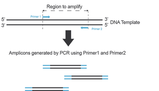
Figure A. Primers anneal to their target on each strand of DNA during PCR and yield amplicons defined by the hybridization location of each primer on the template.
-
Template DNA
Template DNA can be any DNA to be amplified, whether extracted from animal or plant cells, fungi, bacteria, or present in free form- for example circulating DNA in blood or urine. For optimal results, it is recommended to use long-enough purified DNA fragments for amplification to take place. Additionally, caution needs to be exercised to avoid chemical and/or UV-induced damage to the DNA template as it may affect your PCR results.
2. Thermal Cycling in PCR
PCR is based on thermal cycling: the reaction mix is subjected to sequential cycles of heating and cooling, which allow specific temperature-dependent reactions to occur.
-
Denaturation
First, DNA is denatured or melted at a high temperature, typically 94-96°C. During this step, the hydrogen bonds between complementary bases of the double-stranded DNA are broken, yielding two single-stranded molecules. Depending on the type of DNA, the reagents, and equipment used this step usually lasts ranging from 15 seconds to 1 minute and marks the start of each cycle of PCR.
-
Annealing
After denaturation of the template DNA strands, primers anneal to their target on the DNA template. The temperature of this step is critical to ensure specific hybridization of the primers to the target. In practice, this temperature is usually determined empirically- it needs to be low enough to allow primer binding but high enough for the binding to be specific to the intended target. Usually, annealing temperatures are between 3-5°C below the calculated Tm of primers, which translates to annealing temperatures for PCR between 50-65°C. Once the primer has annealed to the DNA, the polymerase binds to the primer-template hybrid and elongation can start.
-
Elongation
During elongation, the polymerase synthesizes new DNA strands by adding free nucleotides (dNTPs) present in the PCR reaction one-by-one, and the polymerization of the new strand complementary to the template takes place in the 5’ to 3’ direction
The temperature for elongation depends on the polymerase used, with 68-72°C being most commonly used. The length of the amplicon is taken into account when determining the time needed for the elongation step with a general rule of thumb of 1 minute per kb to be synthesized. The synthesis rate of the polymerase present in your PCR mix can be found in the manufacturer’s recommendation.
-
Additional steps
Initial denaturation
Before cycling starts, a longer initial denaturation step is often included (90-95°C for 1-10 minutes). Why? Because hot-start polymerases must be activated as these enzymes have been developed to reduce non-specific amplification early in the PCR reaction. Thus, they are locked in an inactive state by binding to an antibody or a chemical inhibitor. At elevated temperatures, a non-reversible dissociation occurs and this unlocks the enzyme.
Final Elongation
A final extension step (68-72°C for 5-10 minutes) can also be included to ensure all amplicons are fully elongated.
3. What happens during PCR?
-
Number of copies of target DNA fragment generated during PCR
If the reaction efficiency is 100%, the number of amplicons doubles after each cycle. This means that each copy of the DNA target initially present will be amplified 2n, where n is the number of cycles of PCR. Thus, when amplifying a single copy of your target region for 40 cycles, you could finally get 240 = 1.1 x 10¹² amplicons!
-
Stages of PCR
Given that the number of amplicons doubles at each cycle when PCR efficiency is 100%, PCR amplification is referred to as exponential.
However, since this is an enzymatic reaction one or more factors will become limiting as the reaction progresses. Moreover, the polymerase may also start to lose activity. This will mean that at some point the amplification will start to level off, before reaching a plateau where no more products are generated.
4. How are the PCR results visualized?
-
Electrophoresis
Traditionally, the products of PCR are run on an agarose gel to visualize the amplicons. The agarose gel is stained with an agent that will bind to DNA (ethidium bromide or GelRed® for example) and illuminated with UV light in order to reveal the various DNA fragments present. Typically, a DNA ladder is run alongside the PCR products to estimate the size of the products, as well as the amount of DNA generated (Figure B).
Other electrophoresis techniques may use capillary gels and fluorescently labeled primers for fine discrimination of amplicon size.
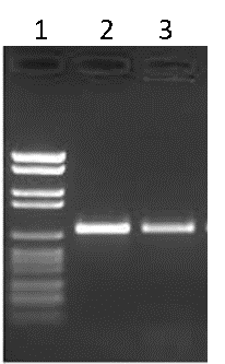
Figure B. Agarose gel electrophoresis. Lane 1: DNA ladder, Lane 2: PCR product 1, Lane 3: PCR product 2
-
Fluorescence
Different chemistries allow the fluorescence detection of DNA molecules. Amongst these chemistries, Hydrolysis probes, SYBR® Green I, and EvagGeen® are the most commonly used.
Hydrolysis probes (TaqMan® probes)
A probe, like primers, corresponds to a short oligonucleotide sequence (different from primer sequences) complementary to the target DNA sequence. Located between the sense and anti-sense primers, the hydrolysis probe consists of a fluorescent dye and a quencher. During amplification, the hydrolysis probe will be cleaved by the 3’->5’ exonuclease activity of the Taq polymerase. This will separate the fluorescent moiety from its quencher (Figure C). These fluorescent molecules will accumulate after each cycle. A fluorescent signal proportional to the number of amplicons bearing the probe hybridization sequence can be recorded. If you want to know more about probes, refer to the “Designing Primers and Probes” item.
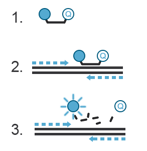
Figure C. Hydrolysis probes. 1. The probe is a single-stranded DNA sequence labeled with a fluorophore at its 5’ end and a quencher at its 3’ end. The fluorescence of the fluorophore is quenched, i.e., absorbed by the quencher- no light is emitted. 2. During PCR, the probe will hybridize with the amplicon generated in a sequence-specific manner. 3. The 3’ to 5’ exonuclease activity of the Taq polymerase destroys the hybridized DNA probe, thus freeing the fluorophore from the quencher. This fluorophore is now free to emit a fluorescent signal.
DNA-binding dye: EvaGreen®
EvaGreen® is a DNA binding dye that can be used to track PCR amplification in most digital PCR systems. It is a green fluorescent dye which becomes highly fluorescent when it is bound to double-stranded DNA. EvaGreen® is a thermoresistant molecule with excitation and emission spectra close to that of SYBR® Green I or 6-FAM dyes. Please note that the advantage of EvaGreen® over SYBR® Green I is its compatibility with droplet-based digital PCR systems. Thus, SYBR® Green I is mostly used in real-time PCR.
When using EvaGreen, the intensity of the fluorescent signal will correlate with the length of the amplicon generated. The longer the amplicon, the more bases available for EvaGreen binding, thus the stronger the fluorescence signal (Figure E).
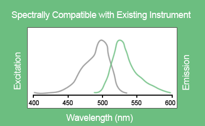
Figure D. Excitation and emission spectra of EvaGreen® in the presence of double-strand DNA in PBS buffer
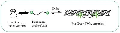
Figure E. EvaGreen® dye binds to double-strand DNA via a “release-on-demand” mechanism.
[https://biotium.com/technology/pcr-dna-amplification/evagreen-dye-for-qpcr/]
Fluorescence detection is the detection system used both in digital and real-time PCR.
Further information about EvaGreen® can be found on the manufacturer’s website
Digital PCR
Most digital PCR platforms use end-point PCR for quantification. End-point PCR means that the results of PCR are assessed when the plateau is reached. It occurs when the amplification has stopped due to loss of polymerase activity or an essential reagent (primers for example) present in the reaction.
In these reactions, fluorescent reporters are used. It can be DNA-binding dyes such as EvaGreen or fluorescently-labeled hydrolysis probes.
For further information on digital PCR refer to the “Principle of Digital PCR” item.
Real-time PCR
The intensity of the fluorescent signal is recorded at each cycle of PCR. The results are visualized on a graph where the intensity of fluorescence is plotted against the number of cycles. During the first few cycles, the fluorescent signal generated by the fluorescent reporter is indistinguishable from the background. As amplification takes place during cycles, the fluorescence eventually increases above noise level before tailing off and reaching a plateau.
Due to the accumulation of amplicons, the exponential increase of fluorescence can be visualized on the graph. A threshold for fluorescence intensity is placed at the beginning of this exponential phase. The cycle number at which the amplification curve intersects the threshold is called Cq (Cycle quantification). The quantification of an unknown sample assumes the use of a standard curve. By comparing the Cq obtained for DNA samples of known concentration with the Cq obtained for the unknown sample, DNA concentration in the unknown sample is then determined (Figure F)
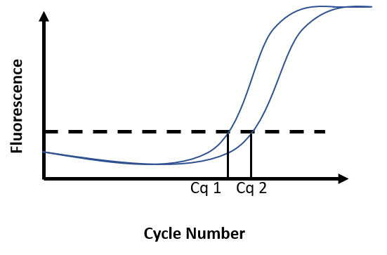
Figure F. Real-time PCR results. Fluorescence intensity is recorded at every cycle and plotted against the cycle number. Reaction 1 has a known DNA concentration (Cq1). At 100% efficiency, the DNA content in the reaction doubles at each cycle. Broadly, if Cq2 is distant from Cq1 from 1 cycle, this means there was half as much DNA in reaction 2 as there was in reaction 1 at the start of the PCR.
Designing Primers & Probes
Primer and probe design is a crucial step for a successful experiment.
The rules for designing primers and probes in a digital PCR assay are similar as for a qPCR assay:
1. Primers
Their length should be between 18 and 25 base pairs.
The criterion that you have to carefully monitor are:
- Percentage of GC: 40-60%
- Primer melting temperature (Tm): ideally between 55-65°C and Tm between both primers should not differ by more than 5°C
- G or C bases at the 3′ of the primer but not more than 2 in the last 5 bases
- Low probability of dimer or hairpin formation
2. Probes
The length should not exceed 30 base pairs. Ideally 15 base pairs for optimal specificity.
The criterion that you have to carefully monitor are:
- Percentage of GC: 20% to 80%
- Probe melting temperature: ideally from 4 to 10°C above the primer melting temperature
- Absence of more than 4 G repeats
- Low probability of dimer or hairpin formation
- Absence of G at the beginning of the probe
Sometimes, you will need to increase the Tm of the probe while keeping its size short. You can use modified bases such as locked nucleic acid (LNA) bases or peptide nucleic acid (PNA) bases. A probe with a minor groove binder (MGB) group is also an option to increase the Tm.
For further information about probe design, please refer to the following publications:
- Design of primers and probes for quantitative real-time PCR methods. Rodríguez A, Rodríguez M, Córdoba JJ, Andrade MJ, Methods Mol Biol. 2015;1275:31-56. doi: 10.1007/978-1-4939-2365-6_3. [PMID: 25697650]
- http://media.axon.es/pdf/78099_2.pdf
More information about MGB group, LNA, and PNA bases:
- Locked nucleic acids in PCR primers increase sensitivity and performance. Ballantyne KN, van Oorschot RA, Mitchell RJ. Genomics. 2008 Mar;91(3):301-5. doi: 10.1016/j.ygeno.2007.10.016.[PMID: 18164179]
- An introduction to peptide nucleic acid. Nielsen PE, Egholm M. Curr Issues Mol Biol. 1999;1(1-2):89-104. Review. [PMID: 11475704]
- https://academic.oup.com/nar/article/28/2/655/1039630
Tools for primer and probe designs:
3. How should I prepare my PCR mix?
Please note that the following protocol has been optimized on the Naica™ System and the Sapphire chip.
a. Importance of DNA preparation and DNA input
Once your DNA has been extracted and purified, you have to calculate the amount of DNA you need to put in your reaction. This will determinate the sensitivity of your assay.
To do so remember in digital PCR we speak in terms of copies of DNA. The following formula will allow you to make the conversion:
Number of copies in reaction volume = mass of DNA in reaction volume (in ng)/0.003
Why 0.003? In this experiment, we are working with human genomic DNA: its mass is approximately 3 pg (=0.003 ng) per haploid genome, and we want to detect the EGFR gene which is present as one copy per haploid genome. If you are working with plasmids or other genomes, you will need to change this value.
Let’s do the math together with the following example, and you will understand how DNA input and sensitivity are related:
- Let’s say that we are working with a DNA input of 10ng (V = 1µL). With the Naica™ System and the Sapphire chip, the total PCR mix volume recommended is 25µL. By applying the formula in the section above, we can say that we are adding: 10/0.003 = 3,333 haploid genomes or copies of EGFR to our mix, meaning 3,333/25 = 133 copies of EGFR/µL as final concentration in the reaction well.
- Depending on the system used, the theoretical limit of detection may vary. With the Naica™ System, the lowest concentration theoretically detectable (theoretical LOD) with 95% confidence level is 0.2 copies/µL.
- Thus, to calculate the lowest theoretical sensitivity for this given sample with 95% confidence interval, we simply divide the theoretical LOD of the system by the total concentration of EGFR copies in our sample:
- Sensitivity = 0.2/133 = 0.15 %
In conclusion, with 10ng of human genomic DNA in your well and when using a digital PCR system with a 0,2 copies/µL theoretical LOD, you should be able to detect a mutated allelic fraction for EGFR down to 0.15 % with 95% confidence, but not lower.
For more details, please check “DNA preparation for Digital PCR” and “Digital PCR assay optimization” items.
b. One more step before starting to manipulate: prepare your working sheet
If you are a qPCR user, the protocol for preparing the PCR mix is the same.
Here is what you need to know:
- How many samples do you want to run: for n=7 samples, in order to take into account volume lost with pipetting error, prepare a total volume of PCR mix for n+1=8 samples.
- What are the manufacturer’s instructions for each component of the PCR mix
Once you are ready, prepare your PCR mix as follows:
Table 1: PCR mix
| Reagents | Final Concentration |
|---|---|
| PCR Mastermix (2X or 5X) | 1X |
| Reference dye | Please refer to the manufacturer’s instructions |
| EGFR T90 Reverse and Forward primers | 500 nM |
| EGFR T790WT probe | 250 nM |
| EGFR T790M probe | 250 nM |
| Human genomic DNA | ”How much DNA input”, see above |
| Water | Up to 25 µL (depending on manufacturers) |
Depending on the type of digital PCR system you are using you may have to generate a compensation matrix, i.e., monocolor controls. In this case, we are performing a duplex assay. Thus, you will need:
- 1 x Non-Template Control (NTC): in this well, you will put all the components of your PCR mix except DNA
- 1 x Monocolor control for EGFR T790WT probe
- 1 x Monocolor control for EGFR T790M probe
This will allow you to correct the fluorescence spillover that may occur between the two fluorophores. Please check the “Fluorescence spillover compensation” item for more details.
In this experiment, we will evaluate the presence of the T790M mutation in 4 samples.
Digital PCR DNA Preparation
DNA preparation is a crucial step for the success of your digital PCR assay. Template extraction, its quality control, and its storage are important parameters to monitor.
-
Template extraction
Digital PCR has been reported to be compatible with DNA & RNA templates extracted by various extraction methods used in laboratory- from phenol chloroform method to modern extraction kits1,2,3,4,5,6
-
Quality control
For optimal digital PCR performance, you should check the purity and the quality of your template. Using relevant methods such as spectrophotometry, you will be able to verify the good absorbance (A260/230 and A230/260) ratios of your extracted DNA solution. The presence of contaminants and/or potential inhibitors should be avoided.
-
Storage
The storage of your extracted DNA template is also an important factor to monitor. Indeed, for example, you need to avoid base degradation such as cytosine deamination and 8-Oxo-2′-deoxyguanosine formation due to oxidative damage since it may lead to base transversion during PCR amplification.
Buffering and temperature conditions have an impact on the quality of your sample. Storing at -20°C in Tris-EDTA is the standard condition, but please do not hesitate to take a look at the extraction kit manufacturer’s recommendations.
Other parameters, inherent to the sample itself, might have an impact on your digital PCR experiment and should be verified :
-
DNA with high GC content
If your template contains a GC-rich region, this might conduct to an incomplete amplification. Indeed, GC bonds are highly stable. Thus, in order to obtain a better denaturation of your template, you can try to add DMSO or betaine in your PCR mix.
-
High molecular weight DNA
High molecular weight DNA or plasmids have been reported by some manufacturers as problematic for partition generation. Thus, we recommend DNA shearing using chemicals or enzymatic methods prior to performing digital PCR. Please note that the digestion step might be performed directly in the PCR mix.
Finally, before starting your digital PCR assay you will have to proceed on the :
-
Conversion of mass of DNA in number of copies
If you are a qPCR user, you may be used to thinking in terms of mass of DNA input.
In digital PCR, you will need to think in terms of the number of copies of genes or genomes in your reaction volume.
In order to proceed on the conversion, the only thing you will have to know is the mass of the studied genome.
Then, simply apply this formula: Number of copies in reaction volume = mass of DNA in reaction volume (in ng)/ mass of the studied genome (in ng)
For more details about how to perform this calculation, refer to Part 3a of Rare Mutation Detection Tutorial.
Online calculators are also available :
- http://cels.uri.edu/gsc/cndna.html
- https://www.thermofisher.com/us/en/home/brands/thermo-scientific/molecular-biology/molecular-biology-learning-center/molecular-biology-resource-library/thermo-scientific-web-tools/dna-copy-number-calculator.html
Bibliography
1 Cai, Y., Li, X., Lv, R., Yang, J., Li, J., He, Y., & Pan, L. Quantitative Analysis of Pork and Chicken Products by Droplet Digital PCR. BioMed Research International, 2014, 810209. http://doi.org/10.1155/2014/810209. PMID: 25243184
2 Pérez-Barrios, C., Nieto-Alcolado, I., Torrente, M., Jiménez-Sánchez, C., Calvo, V., Gutierrez-Sanz, L., Palka, M., Donoso-Navarro, E., Provencio, M., Romero, A. Comparison of methods for circulating cell-free DNA isolation using blood from cancer patients: impact on biomarker testing. Transl Lung Cancer Res. 2016 Dec; 5(6):665-672. doi: 10.21037/tlcr.2016.12.03. PMID: 28149760
3 Demeke, T., Malabanan, J., Holigroski, M., Eng, M. Effect of Source of DNA on the Quantitative Analysis of Genetically Engineered Traits Using Digital PCR and Real-Time PCR. J AOAC Int. 2017 Mar 1;100(2):492-498. doi: 10.5740/jaoacint.16-0284. Epub 2016 Dec 22. PMID: 28118137
4 Holmberg, R.C., Gindlesperger, A., Stokes, T., Lopez, D., Hyman, L., Freed, M., Belgrader, P., Harvey, J., Li, Z. Akonni TruTip® and Qiagen® Methods for Extraction of Fetal Circulating DNA-Evaluation by Real-Time and Digital PCR. PLoS One. 2013 Aug 6;8(8):e73068. doi: 10.1371/journal.pone.0073068. Print 2013. PMID: 23936545.
5 Rajasekaran, N., Oh, M. R., Kim, S.-S., Kim, S. E., Kim, Y. D., Choi, H.-J., Byum, B., Shin, Y. K. Employing Digital Droplet PCR to Detect BRAF V600E Mutations in Formalin-fixed Paraffin-embedded Reference Standard Cell Lines. Journal of Visualized Experiments : JoVE, 2015, (104), 53190. Advance online publication. http://doi.org/10.3791/53190. PMID: 26484710.
6 Devonshire, A. S., Whale, A. S., Gutteridge, A., Jones, G., Cowen, S., Foy, C. A., & Huggett, J. F. Towards standardisation of cell-free DNA measurement in plasma: controls for extraction efficiency, fragment size bias and quantification. Analytical and Bioanalytical Chemistry, 2014, 406(26), 6499–6512. http://doi.org/10.1007/s00216-014-7835-3. PMID: 24853859
Digital PCR Assay Optimization
Sub-optimal digital PCR settings very often lead to insufficient signal to noise ratio. This affects the separation between the negative and the positive partitions and prevents for an adequate threshold setting. That leads to limit the accuracy of the quantification and the sensitivity of the assay.
When developing an assay on a digital PCR system, there are several elements to consider:
- DNA template for assay optimization (positive control)
- Difference in fluorescence amplitude between negative and positive populations
- Presence of partitions of intermediate fluorescence (rain)
- Specificity – Are there non-specific populations? Can you detect positive partitions in your negative control?
1. DNA template for assay optimization
Ideally, the DNA template should be in the same form as it will be in the sample you will want to assay : sheared in small fragments if targeting circulating cell-free DNA or relatively intact if assaying genomic DNA. The DNA solution used should be devoid of contaminants and potential inhibitors and have good absorbance (A260/230 and A230/260) ratios. If there is no evident source for DNA material to develop your assay, you may use synthetic oligos as templates for optimization.
-
Presence of false positives
False positives are also a factor that contributes to the diminution of the sensitivity of the digital PCR assay. To limit this phenomenon, it is crucial to prevent DNA contamination in the laboratory or cross-contamination from well to well. Template quality is also a factor that is important to monitor as base degradation such as cytosine deamination and 8-Oxo-2′-deoxyguanosine formation due to oxidative damage may lead to base transversion during PCR amplification.
For more information about DNA preparation, have a look at the “DNA Preparation For Digital PCR” item.
2. Difference in fluorescence amplitude between negative and positive populations
When you run an assay for the first time, you might not distinguish the negative and positive populations on a digital PCR system (Figure A).
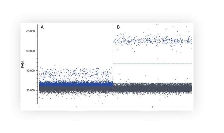
Figure A. The positive partition population (blue) is barely separated from the negative population (dark grey), rendering thresholding difficult on this 1D dot plot. B. The fluorescence of the positive population (blue) is clearly separated from the negative population (dark grey), placing a threshold is therefore unambiguous.
Here are a few tips to improve the separability of your populations:
- Check manufacturers recommendations on primers and probe concentrations to be used in your digital PCR system. These may be higher than the ones usually recommended in qPCR.
- Optimize hybridization temperature. Check for the highest hybridization temperature that gives you an optimal separability and no rain (see below).
- Check the type of probes you are using. Double-quenched probes will give you a lower basal fluorescence signal, and therefore a higher separability.
- Check whether your probes are too old! Depending on how long your probes have been stored, whether they have been stored properly, or whether they just encountered too many freeze-thaw cycles, it is possible that your probes are already hydrolyzed. In this case, you may see a high fluorescence basal level, and, since there are only a few intact probes for PCR, a low signal for the positive partitions.
- If using a system where you can vary acquisition parameters, you may also try to tune the exposure time
3. Presence of partitions of intermediate fluorescence (rain)
We call “rain” partitions that have intermediate fluorescence values between the positive and the negative populations. In these partitions, amplification/hybridization efficiency is sub-optimal. The rain makes the threshold setting harder, and thus may affect quantification.
Various factors may be at the origin of the “rain” such as, template degradation, PCR inhibitors, polymerase errors, primer dimer, target accessibility (Figure B) or non-homogenous distribution of fluorescence into partitions.
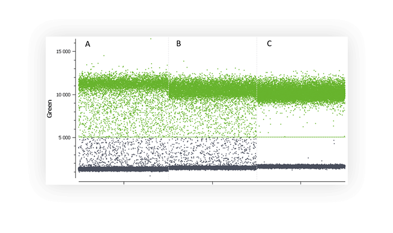
Figure B. 1D dot-plots of a digital PCR experiment in partition using one fluorescent assay targeting a non-digested plasmid (A and B) and a digested plasmid (C). Rain is clearly visible on the two first plot whereas plasmid digestion has removed most of the partitions corresponding to rain.
In order to minimize the rain, you can optimize your digital PCR reaction by:
- Checking the optimal hybridization temperature as described above
- Checking your DNA template for anything that may prevent accessibility to the target. Is this a GC-rich region? Try additives such as DMSO or betaine. When using high molecular-weight DNA or plasmids, it is also best to fragment the DNA by digestion or mechanical means prior to digital PCR. If using digestion, you may also be able to perform this step directly in the mix.
- Making sure to use DNA free from inhibitors
- Increasing the number of cycles in order to ensure that all partitions reach the reaction plateau.
4. Presence of non-expected populations
When assaying a single target, you usually expect a single positive population. But sometimes, you will discover that a second distinct population has appeared (Figure C). It can be due to primer dimers and non-specific amplification.
Multiple fluorescence populations may prevent from setting a proper threshold.
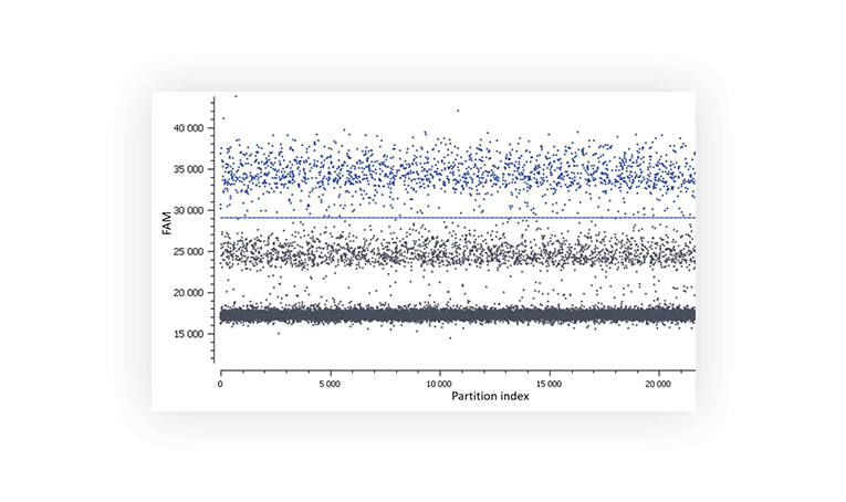
Figure C. In this assay, a second population is observed between the negative (lower grey band) and the positive (blue).
Various methods can be employed to limit this phenomenon such as optimization of primer design, increase of annealing temperature and touchdown PCR.
This specificity issue may be fixed:
- The hybridization temperature is potentially too low so make sure you pick the highest temperature that gives you optimal separability while minimizing the rain
- Have you thought about performing a touchdown PCR?
- Is this non-specific population really an issue ? In terms of quantification, you can just decide to place the threshold above it as we have done in Figure C. The non-specific population amplified will just be considered part of the negative population. The results will thus be calculated only for the amplified partitions that show a reaction efficiency consistent with a specific hybridization of the primers and probes. Please note that this is not the optimal way of analyzing your data since it can have an impact on precision and sensitivity.
- Re-design your primers. To do so, you may use online tools to check that your primers and probes do not hybridize elsewhere in the genome.
For more information on optimization to improve your digital PCR assay, see the following article:
Lievens, A., Jacchia, S., Kagkli, D., Savini, C., Querci, M. Measuring Digital PCR Quality: Performance Parameters and Their Optimization. PLoS One. 2016 May 5;11(5):e0153317. doi: 10.1371/journal.pone.0153317. eCollection 2016. PMID: 271494
c. Everything is ready: hands-on part!
Prior to preparing your PCR mix make sure you are working in a clean area in order to avoid all sources of DNA contamination. The use of a PCR hood is recommended. Assemble the PCR mix based on your working sheet. Make sure all the components are well homogenized before loading the PCR mix into the consumables used for partitioning.
Finally, the hands-on protocol will vary according to your digital PCR system. Please check the manufacturer’s instructions. If you are using the Naica™ System (Stilla Technologies) or the QX200™ Droplet Digital™ PCR System (Bio-Rad), you can check the “Performing Digital PCR Hands On” item.
Performing Digital PCR Hands-On
Each digital PCR platform has its own hands-on protocol. In this item, we have chosen to describe protocols used on the Naica™ System and on the QX200™ Droplet Digital™ PCR System.
For both systems, we will assume that you have already prepared your PCR mix and divided it into 8 tubes: one per sample. You have also loaded your 8 samples.
1. Naica™ System:
Since the Sapphire chips are already prefilled with oil, you have only one last step before launching the PCR reaction.
To do so, you will need :
- 2 Sapphire Chips
- tips and pipette adapted for 25 µL
- 8 tall white caps (provided in the Sapphire Chips box)
Ready? Let’s go!
- Unpack the Sapphire Chips and remove the white caps
- Gently pipette your 25 µl of PCR mix containing your samples into each inlet port
- Finally, seal each inlet port with the tall white caps
The hands-on part is done and you are now ready to place your Sapphire Chips into the Naica™ Geode where the partition generation and the thermal cycling will occur.
A short movie of the workflow is also available here!
2. QX200™ Droplet Digital™ PCR System:
Here, we describe the manual protocol. A faster way to proceed would be to use the QX200™ AutoDG™ Droplet Digital™ PCR System where the following steps are automated and integrated.
Two more steps before launching the PCR reaction :
A. Partitions generation
To do so, you will need :
- 1 x DG8™ Cartridges for QX200™/ QX100™ Droplet Generator
- 1x DG8™ Cartridges holder for QX200™/ QX100™ Droplet Generator
- 1 x DG8™ Gasket for QX200™/ QX100™ Droplet Generator
- 1 x QX200™ droplet generator
- 1x Droplet Generation Oil for Probes
- Rainin pipettes and tips adapted for 20µL and 70 µL
Ready? Let’s go!
- Take the DG8™ Cartridges holder for QX200™/ QX100™ Droplet Generator. Open it by pressing the latches in the middle and sliding the two parts. Place one cartridge inside. Slide again in the original position to close
- Pipette your 20µL of PCR mix containing your sample in the middle wells of the cartridge. Then, pipette 70µL of droplet generation oil in the bottom wells
- Close the cartridge with one dedicated gasket
- Open the QX200™ Droplet generator by pressing the button on the top. Place the cartridge holder and close the droplet generator by pressing again the button
Partitions are now generated! The second and last hands-on part starts now :
B. Partitions transfer
To do so, you will need:
- 1 x ddPCR 96-Well Plate
- 1 x Pierceable foil plate seal
- 1 x PCR plate sealer
- Rainin pipettes and tips adapted for 40 µL
Let’s finish!
- Recover the DG8™ Cartridges holder from the Droplet Generator and remove the gasket. Do not open the cartridge holder.
- Gently pipette the 40µL of generated emulsion (top wells of the cartridge) and smoothly deliver it into a ddPCR 96-Well plate.
- Place the Pierceable foil on the ddPCR 96-well plate and proceed to the sealing part in the PCR plate sealer.
- Finally, place your ddPCR 96-well plate in the thermal cycler and launch your ddPCR program.
4. What are the next steps to get my results?
a. Thermal cycling
The EGFR assay used in this example was optimized using the QuantaBio PerfeCTa Multiplex mastermix, on the Naica™ System (Stilla Technologies). In the table below, you will find the thermal cycling program used for the assay. If you are using a different mastermix or digital PCR system, you may have to optimize this protocol. For more details, please check “Digital PCR assay optimization” item.
Table 2: EGFR T790M assay cycling conditions
| Cycles | Temperature | Time |
|---|---|---|
| 1 | 95°C | 10 min |
| 45 | 95°C | 30 s |
| 62°C | 15 s |
b. Data acquisition
Depending on the system used, data acquisition will take the form of imaging a chip (Naica™ System, QuantStudio™ 3D Digital PCR System, CONSTELLATION® digital PCR system,etc.), or reading partitions one-by-one in a process analogous to flow cytometry (QX200™ Droplet Digital™ PCR System, Raindrop™ Digital PCR System). Please follow manufacturer’s instructions on how to perform this step.
5. How should I analyze my data?
First of all, let us remind you of the usual graphical representation in digital PCR experiments are 1D-, 2D-, or 3D-dot-plots depending on the number of targets you are looking for.
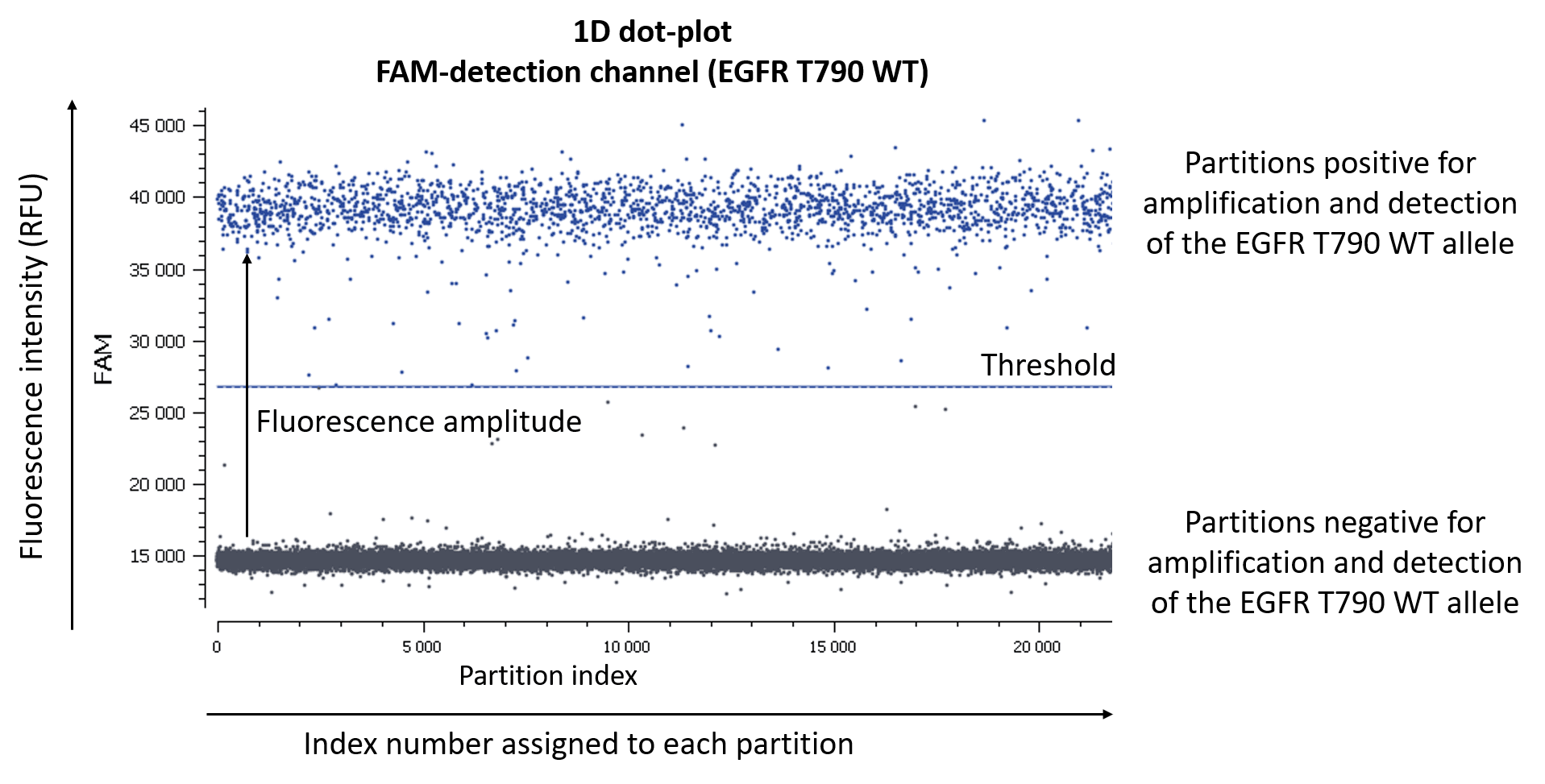
Figure 2. One simple way to visualize data in digital PCR experiments is by using a 1D dot-plot, in which each dot represents one partition. The y-axis gives the fluorescence intensity of each partition in a given detection channel, while the x-axis gives the index number assigned to each partition by the analysis software.
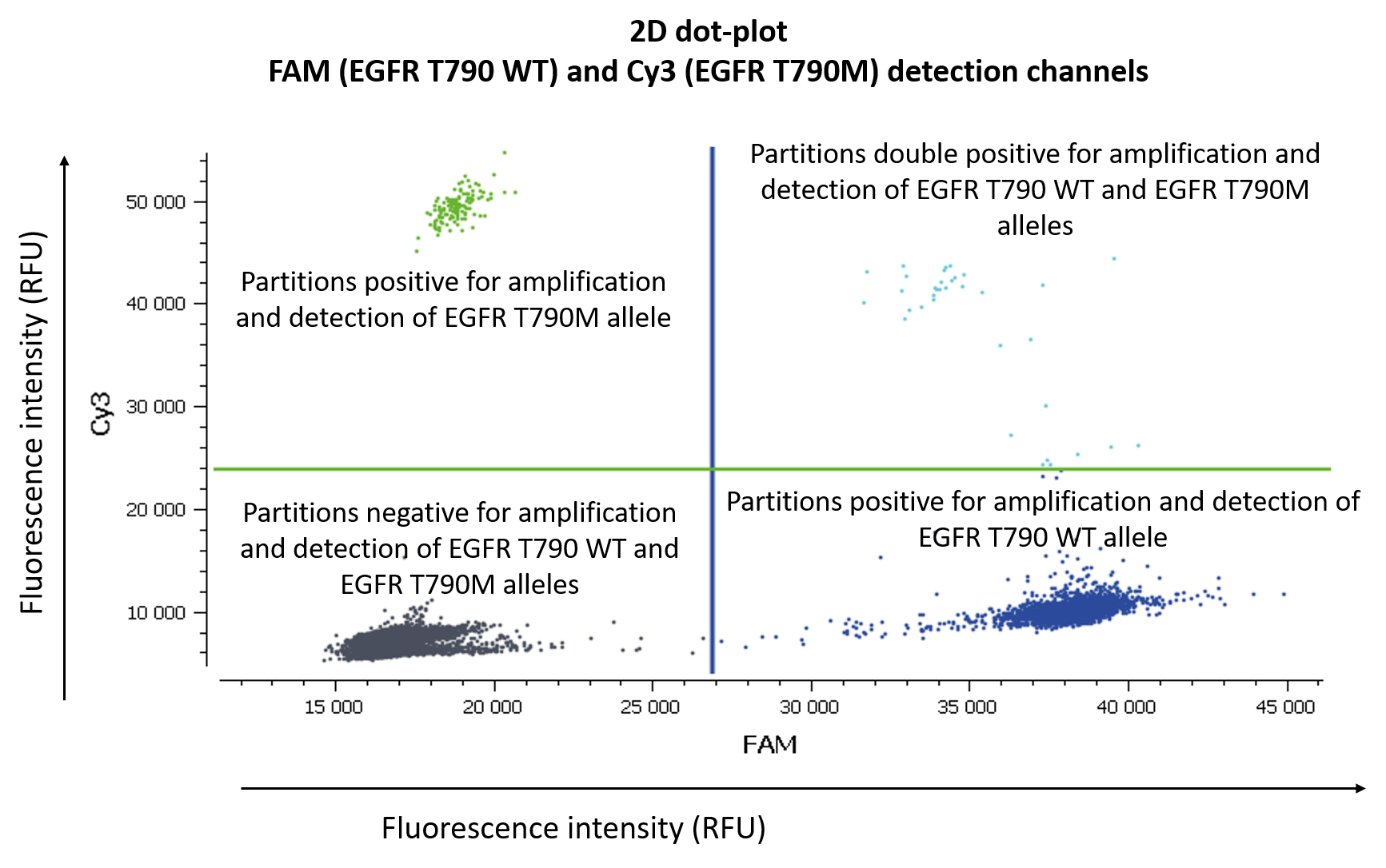
Figure 3. Here two targets are represented, the wild-type and the mutant. Both can be visualized simultaneously in a 2D dot-plot. The y-axis gives the fluorescence intensity of each partition in the Cy3 detection channel, while the x-axis gives the fluorescence intensity of each partition in the FAM detection channel.
If you are looking for 3 different targets, a 3D dot-plot graph will allow you to visualize the different clusters in the 3D space.
a. Quality controls
Depending on the type of data acquisition, data analysis software can present different quality controls. Two criteria should be carefully considered:
- Check the NTC, any or very few positive partitions are accepted. As you can see in figure 4, our NTC presents only negative partitions
- Check the total number of analyzed partitions. Since we are looking for a rare mutation, we can say “the more, the better”. Indeed, with a high number of analyzable partitions, you increase the chance to detect and quantify a rare event, and you decrease the uncertainty associated with the measured concentration. In this assay (table 3) we obtained between 19,000 and 22,000 partitions, validating our experiment
b. Spillover compensation: not available on all digital PCR platforms
When performing multicolor digital PCR experiments, you may encounter fluorescence spillover. This physical phenomenon may be misleading and may yield aberrant results. Thus, you must apply a compensation matrix to the results.
In figure 3, Cy3 fluorescence (coming from EGFR T790M probe), normally detected in the green channel, is causing a second cluster in the Blue channel because Cy3 is partially excited by the blue light source. You can also expect to visualize the detection of the FAM fluorescence (coming from the EGFR T790WT probe and normally detected in the blue channel), in the green channel because FAM is partially excited by the Green source. In figure 5, we can also observe a non-orthogonal disposition of the clusters on the 2D dot-plot. By indicating the wells containing monocolor controls to the software, the matrix compensation will be automatically generated and can be applied to your data.
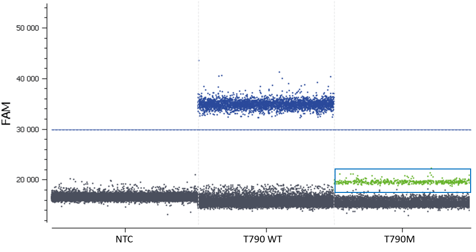
Figure 4. This 1D dot-plot graph represents the fluorescence spillover that may occur between the blue and green channels in monocolor controls. In the T790M well- two different clusters, the negative and the green partitions, corresponding to the detection of the Cy3 fluorescence (in the blue rectangle) coming from the T790WT probe. Please note that no positive partition has been detected in the NTC.
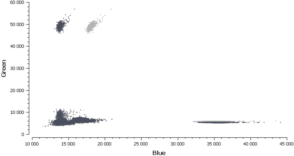
Figure 5. Before applying the compensation matrix, a non-orthogonal disposition of the different clusters (light grey) on the 2D dot-plot graph can be observed. These clusters present the wells containing monocolor controls to the analysis software which adjusts the fluorescence spillover and subsequently the position of the clusters (dark grey).
Once the fluorescence spillover has been corrected, we can proceed to the next step- analysis of patient samples.
Fluorescence Spillover Compensation
Nowadays, all digital PCR instruments available on the market provide multiplexing capability with at least two different detection channels. Fluorescence experiments using multiple fluorophores are commonly set up to detect a unique fluorophore per acquisition channel. However, depending on the fluorophore used, as well as the specifications of the instrument used for acquisition, the signal from a given fluorophore may be detected in more than one channel. This is designated as fluorescence spillover (also called bleedthrough or crosstalk) and it can be encountered in other techniques using fluorescence such as microscopy, real-time PCR or FACS.
Some digital PCR instruments will automatically perform the correction of this phenomenon by applying the same correction factor on all your different experiments. On the other hand, some digital PCR platforms will allow you to create your own compensation matrix. This can be very useful since fluorophores can behave differently depending on their environment.
-
Understanding Fluorescence Spillover
To understand what is happening in fluorescence spillover, let’s consider 2 fluorophores with overlapping excitation and emission spectra, such as FAM and Yakima Yellow.
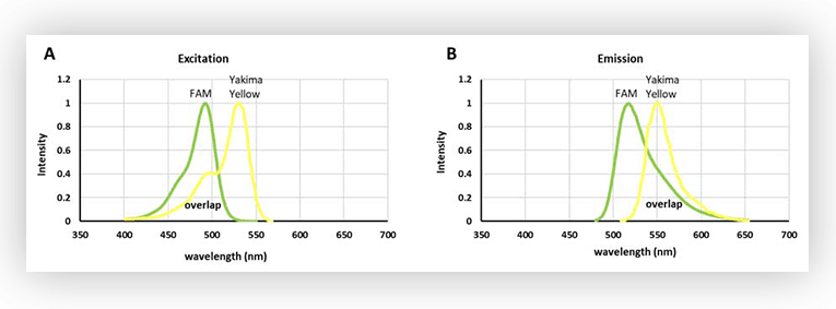
Figure 1. A. Excitation spectra of FAM and Yakima Yellow. B. Emission spectra of FAM and Yakima Yellow.
As shown in Figure 1, there is an extensive overlap between the excitation spectra of FAM and Yakima Yellow. In fact, Yakima Yellow can be excited at almost any wavelength used to excite FAM, although to a lesser extent. So, this means that Yakima Yellow will fluoresce when a light source for exciting FAM is used.
However, set ups for fluorescence acquisition are usually equipped with filters to discriminate the signal. So even if Yakima Yellow is fluorescing, it is possible to acquire only the fluorescence stemming from FAM, by using a narrow filter, at wavelengths where Yakima Yellow fluorescence is marginal (Figure 2.B). An alternative is to have a filter with a wider bandpass (Fig.2.D), thus harvesting more fluorescent signal from FAM, and correcting the interfering signal from Yakima Yellow in post-processing.
As the numbers of fluorophores increase within an experiment, overlap between spectra is practically unavoidable, hence it is important to consider the post-processing correction, called fluorescence spillover compensation.
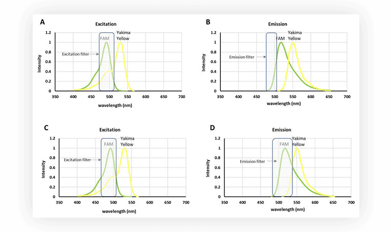
Figure 2. A. Excitation spectra of FAM and Yakima Yellow. B. Emission spectra of FAM and Yakima Yellow. C. Excitation spectra of FAM and Yakima Yellow. D. Emission spectra of FAM and Yakima Yellow. Filters for emission or excitation are represented as light gray rectangles.
-
How can you identify fluorescence spillover in a digital PCR experiment?
Fluorescence spillover can be identified on 2D dot-plots. Indeed, the increase of fluorescence intensity of a positive population in channel 1 correlates with an increase of fluorescence intensity of the same population in channel 2. The result is that the populations are not orthogonal when visualized as 2D. When data is projected on a 1D dot-plot, this means a second population will be present, sometimes rendering thresholding difficult (Figure 3B).
After spillover compensation, the populations are placed orthogonally on the 2D dot-plot, no additional populations appear on the 1D dot-plot, and the thresholds can be readily placed (Figure 3C and 3D).
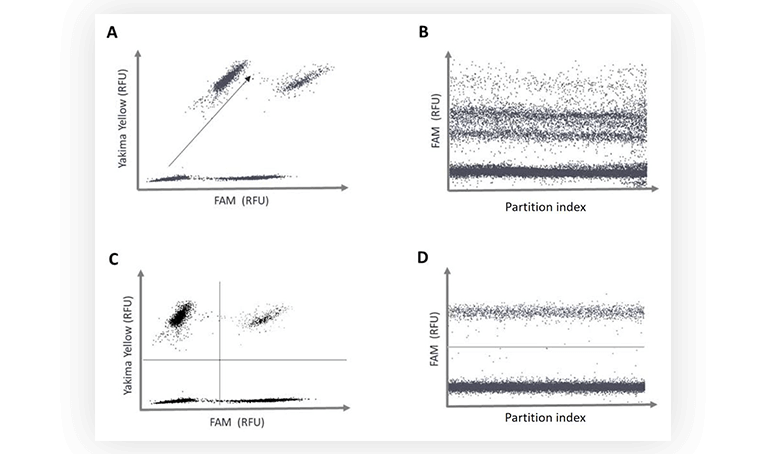
Figure 3. A. and C. Fluorescence intensity of partitions in the channel assigned to Yakima Yellow detection versus fluorescence intensity of partitions in the channel assigned to the detection of the FAM fluorophore. B and D. 1D dot plot. Fluorescence intensity of partitions in the channel assigned for FAM detection versus the partition index. Raw fluorescence data, no fluorescence spillover compensation performed (A and B). Compensated fluorescence data (C and D).
It is important to note that such observations can also stem from a probe cross-specificity issue, or a physical linkage between the targets assayed, hence it is essential to differentiate these biochemical or biological effects from a strictly optical one such as fluorescence spillover.
-
How do you correct the fluorescence spillover?
1.Experimental set-up
Before routinely running your samples with a dedicated assay, you will have to create and save a “compensation matrix”. A compensation matrix allows recovering 2 (or more) fluorescence values emitted by 2 (or more) possible fluorophores contained in a given partition. To do so, you need to run an experiment with wells dedicated to mono-color controls. These controls are used to compensate the fluorescence spillover.
Let’s say you need to build a compensation matrix for an assay with 3 different fluorophores.
You need to prepare 4 different mixes that will be loaded into 4 wells as shown in Figure 4. In each mix, all probes must be included.
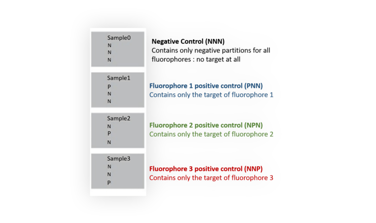
Figure 4. Experimental set-up for building a compensation matrix with a 3-color assay
2. Mathematical correction
The fluorescence readout instrument is typically based on \(M\) fluorescence channels, which means a set of \(M\) detection channels will be used to detect \(M\) standard or custom fluorophores.
We assume that the main detection channel of the fluorophore \(k\) is the source \(k\). The partial excitation of the fluorophores by the sources can be represented by the \(M\times M\) excitation matrix \(E\) where:
- \(E(k, k) = 1\)
- \(E(i, j)\), with \(i \ne j\), is an excitation percentage representing the partial excitation of the fluorophore \(i\) by the source \(j\)
In order to recover the vector \(X\) of \(M\) fluorescence values emitted by the \(M\) possible different fluorophores contained in a given partition, a compensation matrix should be applied to the vector \(Y\) of \(M\) fluorescence values recorded for this partition. This compensation matrix is a transformation which transfers the \(M\) partition coordinates from the “Light domain” to the “Fluorophore domain”.
The resulting spill-over formula is:
- \(X=inv(E) \ (Y – T) + T \)
where:
- \(inv(E)\) is the inverse of the excitation matrix \(E \)
- \(T\) is the translation vector corresponding to the background fluorescence of the partition
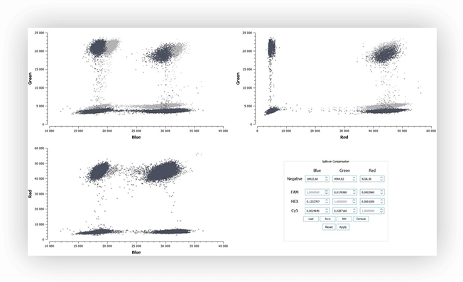
Figure 5. Example of a fluorescence spillover compensation including M = 3 fluorescence channels, with 2D dot-plots of partition fluorescence values (light gray: before compensation; dark gray: after compensation), and the associated 3×3 excitation matrix E.
To conclude, when performing digital PCR experiments with 2 or more fluorophores, make sure that fluorescence spillover is corrected for, whether through hardware or post-processing, depending on the instrument used. If unsure, please contact your manufacturer for more information on how fluorescence spillover is dealt with.
c. Threshold setting
Usually, the threshold is automatically set by the analysis software using a clustering algorithm that maximizes (resp. minimizes) inter-cluster (intra-cluster) point-to-point distances. Partitions above the threshold are positive and those under the threshold are negative. Setting the threshold is thus, a mandatory step to process and accurately quantify the samples.
Since the threshold setting is an automated calculation, we advise you to have a look at the dot-plots.
Note:
- When there are a very small number of positive partitions or a very small number of negative partitions, the threshold has to be manually set.
- When you observe a lot of partitions between the positive and the negatives ones (a phenomenon called “rain”), you might have to adjust the threshold (please note that you might also consider optimization of your assay if the rain is really important).
- When there is a cross-reactivity between probes, you can observe more clusters than expected. Make sure that these clusters are not coming from fluorescence spillover, by applying the compensation matrix if the software offers this option. Then, according to the result obtained, adjust the threshold.
In this experiment, the threshold has been correctly set by the analysis software (figures 6, 7). For more details, see the Advanced Threshold Setting item.
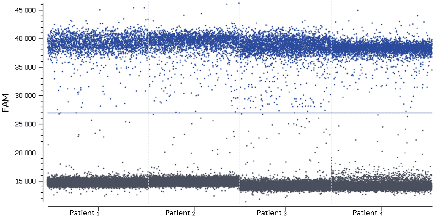
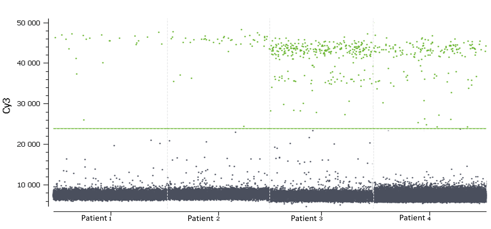
Figure 6. 1D dot-plots in blue (above) and green (below) channels for all wells, each one representing a patient sample. The threshold is represented by a blue line in the blue channel and by a green line in the green channel. The negative and positive partitions are clearly separated in both channels so the analysis software was able to correctly set the automated threshold.
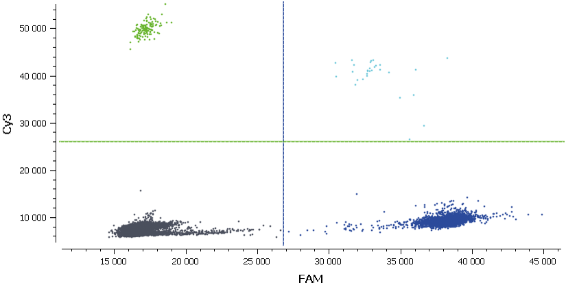
Figure 7. Here, we are looking at the 2D dot-plot graph for the sample corresponding to patient number 4. Once again, we can observe the orthogonal position of the different clusters. Since a 2D dot-plot graph represents the fluorescence intensity of each partition in the blue and the green channels, the threshold of both channels is represented by green and blue lines. The different populations of partitions are well separated so there is no ambiguity on the result of the automated threshold setting.
d. Calculating target concentration
After the correct threshold setting, the software automatically quantifies the number of positive and negative partitions for each target. This digital readout is then converted to a result displayed as the number of copies of the target per microliter using the Poisson distribution.
Thanks to the Poisson distribution, each result will be provided together with a 95% confidence interval which reflects the precision. The accuracy of the measure can also be given by the “95% Confidence interval” value. The smaller, the better!
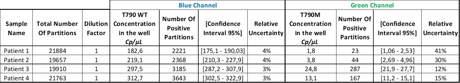
Table 3. For each sample and for each target, the concentration, its 95% interval of confidence, and its associated relative uncertainty will be automatically calculated by the analysis software. Here, the dilution factor is 1 so the data obtained is the concentration in the well. Please note that if you prefer to obtain the concentration in your stock solution, do not forget to correct this value by your dilution factor.
We now have the result table of the experiment but this does not mean that the analysis is done!
Advanced Threshold Setting
When the different populations are not well separated, automatic thresholding fails and must be manually adjusted. The threshold is usually set using horizontal or vertical bars.
- When a single fluorophore assay is used, the 1D dot-plot enables manual threshold setting:
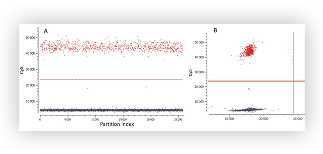
Figure A. 1D plot (A) and 2D plot (B) of a digital PCR experiment with a simplex assay. The positive and negative populations are well separated and the software has successfully calculated a threshold.
- When two or more fluorescent assays are used, it is advised to visualize the 2D dot-plot of the results to verify if both thresholds are correctly set. Furthermore, the visualization using 2D dot-plot can be useful to understand how populations are distributed.
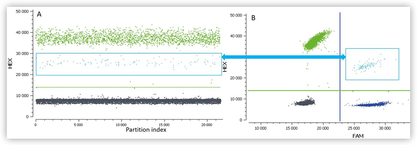
Figure B. 1D plot (A) and 2D plot (B) of a digital PCR experiment with a duplex assay (FAM and HEX). The light blue population corresponds to partitions containing one or more targets detected both by the HEX and the FAM assays (double-positive partitions). Due to competition for the PCR reagents in these partitions, the intensity for HEX fluorescence is decreased for the double-positive population. The threshold on the 2D dot-plot must be set to accommodate this intermediate population in the HEX channel.
- Finally, if you need to manually adjust the threshold, do not forget to have a look at the wells containing your positive and negative controls included in each experiment. They provide information that can be useful for threshold setting.
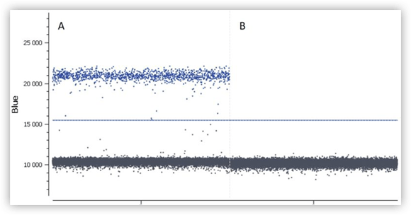
Figure C. Results obtained for positive (A) and a negative (B) controls.
e. Calculating the Limit of Blank and Limit of Detection
For each new assay the Limit of Blank (LOB) and the Limit of Detection (LOD) must be estimated- not only prior to routinely using your assay, but also every time you change your assay as a part of its validation. This step will ensure unbiased results.
Why should I evaluate the LOB? In rare mutation detection assays, sometimes false positives are encountered, i.e. positive partitions for the mutated allele although the sample contains only wild-type templates. In other words, “noise” of the assay. In general, false positive partitions can be due to non-specific hybridization of the mutant probe onto wild-type sequence, polymerase error, well-to-well contamination, environmental contamination, template degradation, or base substitution due to template degradation. The false positive rate is assay dependent. Ideally, it should be zero but false positives can be very difficult to completely get rid of. To evaluate a statistically relevant LOB it is necessary to perform the assay on more than 30 wild-type controls.
For more details about LOB calculation, see the item below about LOB & LOD Definition.
Why should I evaluate the LOD? The LOD is a theoretical value representing the lowest concentration of detectable target in a well with 95% confidence. The larger the LOB, the larger the LOD for your assay.
For more details about LOD calculation, see the item below about LOB & LOD Definition.
The LOB is most frequently expressed as the number of positive partitions within a well. Let’s assume that we are working on an assay for which the LOB is estimated to be 4 positive partitions. After running the assay positive samples are obtained and one of them exhibits 3 positive partitions. In this case, the target is said to be “not detected with 95% confidence level” because it is not possible to say whether the positive signal is from the false positives (noise) or the actual targets present in the sample (signal).
In the EGFR T790WT/M assay, we assayed 32 samples containing WT DNA and calculated the frequency of positive partitions in these samples. Using the LOB calculator tool below, we found that the LOB for this assay was 2 partitions.
Now that you have the LOB, you can assay your samples and detect the EGFR T790M mutation with a 95% confidence level only if the number of positive partitions found in your samples is strictly larger than your LOB. Simply use the online calculators to get a lower-bound estimate of the real concentrations for each sample (Table 4).
The results for rare mutation detection are usually presented in terms of VAF (Variant Allele Frequency), or the percentage of mutation. If the analysis software does not have the option for a VAF result, you can use this VAF calculator.
Table 4. The results obtained in the green channel have been replaced with lower-bound estimates accounting for the LOB.
Finally, in the last column, the VAF for each sample was calculated using the formula “VAF = (Cmut/(Cmut+CWT))”
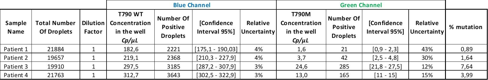
Finally, the last column of the table shows the percentage of mutation for each patient. The oncologists can adjust the treatment based on these results.
LOB and LOD Definition
Before routinely using your digital PCR assay, you should estimate the Limit Of Blank (LOB) and the Limit Of Detection (LOD).
Starting with the LOB, the estimation of the LOD will be then derived from this estimated LOB.
How would you define each parameter?
When the number of positive partitions found in a sample is:
- smaller than the LOB, then the target is said not detected
- larger than the LOB, then the target is said detected
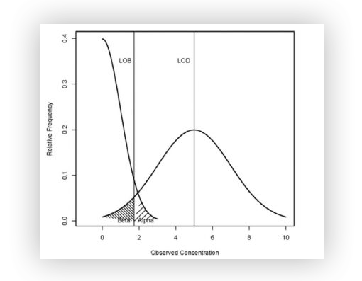
Figure A : Illustration of LOB and LOD
Here are the mathematical definitions of LOB and LOD :
- The Limit of Blank \(LOB\) with a confidence level \((1 – \alpha)\) is defined (in number of partitions) as the maximum number of positive partitions expected in a well with a probability of \(1 – \alpha\) in a sample containing no target sequence.
In other words, it is the maximum number of false positives that are plausible with a \(1 – \alpha\) probability (typically 95% for \(\alpha = 5\%\) of false positives).
To go further on a method to calculate the LOB of a given digital PCR experiment, do not hesitate to have a look at the memo LOB calculation Method.
- The Limit of Detection \(LOD\) with a confidence level \((1 – \beta)\) is defined as the minimum concentration for which detecting the target sequence in a well is possible with a probability of \(1 – \beta\).
In other words, this is the minimum concentration that can be said to be non-zero and statistically higher than the limit of blank \(LOB\) with a \(1 – \beta\) probability (typically 95% for \(\beta = 5\%\) of false negatives).
Knowing the LOB, if you need a method to calculate the LOD of a given digital PCR experiment, do not hesitate to have a look at the memo provided LOD calculation Method.
If you need to automatically compute the LOB and the LOD of a target gene from a set of negative control replicates, an online tool is provided for automated LOB and LOD estimation, let’s try it !
6. To sum up:
- Assay your samples with the conditions set up as described above, or using optimized conditions if using another digital PCR system.
- Check that any fluorescence post-treatment corrections such as spillover compensation are performed.
- Verify that the thresholds are placed adequately on the dot-plots.
- Export results from the manufacturer’s software, making sure to include for each sample: the partition volume, the total number of partitions, as well as the number of positive partitions.
- Subtract the number of partitions found for the LOB from the number of positive partitions in the samples.
- Use online calculators to recalculate the corrected concentrations for each sample.
Congratulations on successfully performing this digital PCR experiment!
Want to discover more dPCR experiments? Check our other tutorials!
MIQE Guidelines
In order to ensure experimental transparency, consistency between research laboratories and thus, maintain a high level of integrity in publications, a guideline for real-time PCR experiments has been edited in 2009 by an international research team [PMID: 19246619].
Considering the increasing number of publications in the Digital PCR field, the MIQE (for Minimum Information for Publication of Quantitative real-time PCR Experiments) guideline has been updated for digital PCR experiments under the name “the Minimum Information for the Publications of Quantitative Digital PCR Experiments guidelines (dMIQE)”[PMID: 23570709].
Having a look at this guideline before starting designing an experiment can be very informative. Indeed, as an example of what you can read in the dMIQE, you will find, below (Table 1), a checklist you might follow for performing a digital PCR experiment. Finally, all items are categorized as essential (E) or desirable (D) for manuscript submission. Thus, citing the following dMIQE in your publication will be a guarantee of quality, for reviewers and readers.
| Table 1. dMIQE checklist for authors, reviewers and editors.a | |||
| Item to check | Importance | Item to check 2 | Importance |
| Experimental design | dPCR oligonucleotides | ||
| Definition of experimental and control groups. | E | Primer sequences and/or amplicon context sequence.b | E |
| Number within each group. | E | RTPrimerDB (real-time PCR primer and probe database) identification number. | D |
| Assay carried out by core lab or investigator’s lab ? | D | Probe sequences.b | D |
| Power analysis. | D | Location and identify of any modifications. | E |
| Sample | Manufacturer of oligonucleotides. | D | |
| Description. | E | Purification method. | D |
| Volume or mass of sample processed. | E | dPCR protocol | |
| Microdissection or microdissection. | E | Complete reaction conditions. | E |
| Processing procedure. | E | Reaction volume and amount of RNA/cDNA/DNA | E |
| If frozen-how and how quickly? | E | Primer, (probe), Mg ++ and dNTP concentrations. | E |
| If fixed- with what, how quickly? | E | Polymerase identity and concentration. | E |
| Sample storage conditions and duration (especially for formalin-fixed, paraffin-embedded samples). | E | Buffer/kit catalogue no. and manufacturer. | E |
| Nucleic acid extraction | Exact chemical constitution of the buffer | D | |
| Quantification-instrument/method. | E | Additives (SYBR green I, DMSO, etc.). | E |
| Storage conditions: temperature, concentration, duration, buffer. | E | Plates/tubes Catalogue No and manufacturer. | D |
| DNA or RNA quantification | E | Complete thermocycling parameters. | E |
| Quality/integrity, instrument/method, e.g. RNA integrity/R quality index and trace or 3’:5’. | E | Reaction setup. | D |
| Template structural information. | E | Gravimetric or volumetric dilutions (manual/robotic). | D |
| Template modification (digestion, sonication, preamplification, etc.) | E | Total PCR reaction volume prepared. | D |
| Template treatment (initial heating or chemical denaturation). | E | Partition number. | E |
| Inhibition dilution or spike. | E | Individual partition volume. | E |
| DNA contamination assessment of RNA sample. | E | Total volume of the partitions measured (effective reaction size). | E |
| Detail of DNase treatment where performed. | E | Partition volume variance/SD. | D |
| Manufacturer of reagents used and catalogue number | D | Comprehensive details and appropriate use of controls. | E |
| Storage of nucleic acid: temperature, concentration, duration, buffer. | E | Manufacturer of dPCR instrument. | E |
| RT (if necessary) | dPCR validation | ||
| cDNA priming method + concentration. | E | Optimization data for the assay. | D |
| One- or 2-step protocol. | E | Specificity (when measuring rare mutations, pathogen sequences etc.) | E |
| Amount of RNA used per reaction | E | Limit of detection of calibration control. | D |
| Detailed reaction components and conditions. | E | If multiplexing, comparison with singleplex assays. | E |
| RT efficiency. | D | Data analysis | |
| Estimated copied measured with and without addition of RT.b | D | Mean copies per partition (ʎ or equivalent). | E |
| Manufacturer of reagents used and catalogue number. | D | dPCR analysis program (source, version). | E |
| Reaction volume (for 2-step RT reaction). | D | Outlier identification and disposition. | E |
| Storage of cDNA : temperature, concentration, duration, buffer. | D | Results of no-template controls. | E |
| dPCR target information | Examples of positive(s) and negative experimental results as supplemental data. | E | |
| Sequence accession number. | E | Where appropriate, justification of number and choice of reference genes. | E |
| Amplicon length. | E | Number and concordance of biological replicates. | D |
| In silico specificity screen (BLAST, etc.) | E | Number and stage (RT or dPCR) of technical replicates. | E |
| Pseudogenes, retropseudogenes or other homologs? | D | Repeatability (intraassay variation). | D |
| Sequence alignment. | D | Reproductibility (interassay/user/lab etc. variation). | D |
| Secondary structure analysis of amplicon and GC content. | D | Experimental variance or Cl.d | E |
| Location of each primer by exon or intron (if applicable). | E | Statistical methods used for analysis. | E |
| Where appropriate, which splice variants are targeted? | E | Data submission using RDML (Real-time PCR Data Markup Language).
|
D |
| a All essential information (E) must be submitted with the manuscript. Desirable information (D) should be submitted if possible.
b Disclosure of the primer and probe sequence is highly desirable and strongly encouraged. However, since not all commercial predesigned assay vendors provide this information, when it is not available assay context sequences must be submitted [Bustin et al. (48)]. c Assessing the absence of DNA using a no-RT assay (or where RT has been inactivated) is essential when first extracting RNA. Once the sample has been validated as DNA free, inclusion of a no-RT control is desirable, but no longer essential. d When single dPCR experiments are performed, the variation due to counting error alone should be calculated from the binomial (or suitable equivalent) distribution. |
|||